cites
Support-Vector Networks
1995
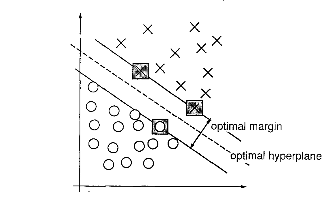
Figure 2. An example of a separable problem in a 2 dimensional space. The support vectors, marked with grey squares, define the margin of largest separation between the two classes.
(Cortes and Vapnik, 1995)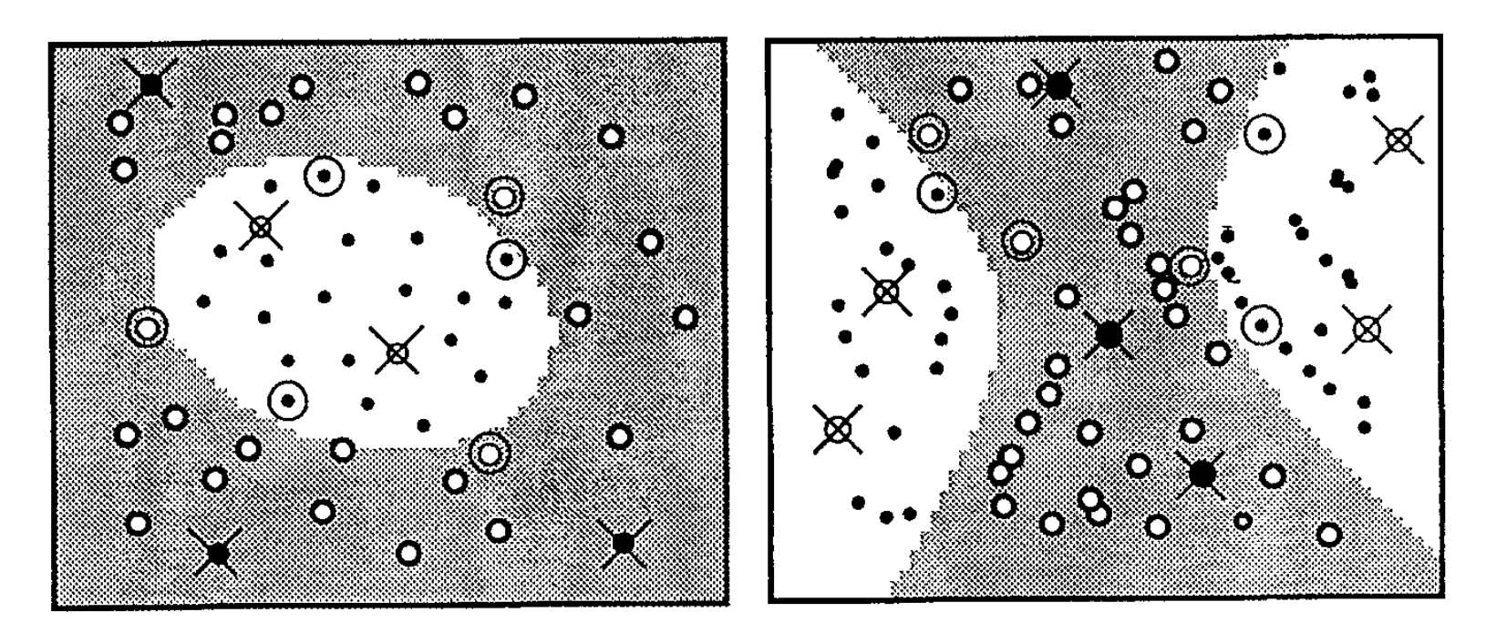
Figure 5. Examples of the dot-product (39) with d = 2, Support patterns are indicated with doable circles, errors with a cross.
(Cortes and Vapnik, 1995)The support-vector network implements the following idea: it maps the input vectors into some high dimensional feature space Z through some non-linear mapping chosen a priori. In this space a linear decision surface is constructed with special properties that ensure high generalization ability of the network.
(Cortes and Vapnik, 1995)Decision boundaries change in two ways in support vector machines. They blur and bend, again affecting what counts as pattern.
(Mackenzie, 2017, p.141)The extravagant dimensionality realized in the shift from 30 to 40,000 variables vastly expands the number of possible decision surfaces or hyperplanes that might be instituted in the vector space. The support vector machine, however, corrals and manages this massive and sometimes infinite generation of differences at the same time by only allowing this expansion to occur along particular lines marked out by kernel functions.
(Mackenzie, 2017, p.147)Cortes, C. and Vapnik, V. (1995) ‘Support-vector networks’, Machine learning. Springer, 20(3), pp. 273–297. [link]
Mackenzie, A. (2017) Machine Learners: Archaeology of a Data Practice. MIT Press.
cites